402 Agency · AI research since 2017 · Technical University of Sofia · Faculty of Computer Systems and Control · Bachelor's thesis · 19 September 2017
Design and Implementation of an Application for Visualisation and Interpretation of Game Artificial Intelligence
Original title: „Дизайн и реализация на приложение за визуализация и интерпретация на игрови изкуствен интелект“. English showcase edition, prepared in 2026 from the 48-page Bulgarian original.
About this edition. This is an English presentation of the thesis, not a word-for-word translation. The author's own material is kept in full: the environment design, the game mechanics and their physics, the choice of learning method, the exploration strategy, the implemented classes, the usage instructions, the experiments and the conclusion. The background sections that summarised public reference material (what Python, pygame, virtualenv and neural networks are) are shortened. Figure and table numbers follow the original so the two can be read side by side.
Screenshots and result graphs are reproduced from the original PDF. The author's schematic figures (the map, the coordinate system, the three force diagrams, the redraw diagram) are redrawn as vector graphics with their labels translated, keeping the original geometry. Figures the original took from public sources (the MDP graph, the Q-learning formula image, the Q-table tutorial, the neuron and network diagrams, the DeepMind results chart, the trends charts) are redrawn or described. Where the edition departs from the original text, an editor's note says so.
Introduction
Original page 4
When writing software, the developer's task is to create an algorithm whose execution solves a given problem. As the problem grows harder, it becomes harder to think up the exact steps that solve it in every scenario. This kind of problem appears, for example, in game development when a bot opponent has to be created. The bot must be able to take decisions that lead to a favourable end of the game for it. When the game has a huge number of states and a large number of actions, it is nearly impossible for a software engineer to foresee every case and write a "static", hard-coded algorithm for the bot to play by. In such cases artificial-intelligence algorithms are appropriate. Put simply, these are mathematical functions or models which, given enough data, manage to "learn" the actions that lead to the greatest reward.
Despite their effectiveness, these algorithms lack clarity about how they actually work, how they could be improved and what weaknesses they have. With a graphical representation of the models we can analyse their results, and compare several models against one another graphically. That makes us more confident in how they act and in their ability to take decisions.
In this thesis I develop both the problem and its solution, together with an analysis and interpretation of the effectiveness of the model that was built. Specifically, the application consists of:
- A test simulation environment (a game).
- An artificial-intelligence model.
- Graphical analysis of the model.
The problem and existing solutions
Original page 5
The core of the problem is the development of the artificial-intelligence model. Once developed it can easily be reused in other environments, for example the OpenAI Gym platform, developed by a team founded by Elon Musk and Sam Altman. With small modifications it can be reused for any problem that reinforcement learning can solve; autonomous cars are one such problem.
Because the range of applications is so wide, many models and libraries exist. Since the model in this thesis solves a problem built for this application, there is no directly existing solution. The available frameworks can still be considered. The most widely used is TensorFlow, a community-developed set of classes and methods built on data flows and graphs, whose nodes are mathematical functions; common structures, optimisers and preprocessors come ready for the developer. Others are Theano, Torch, Infer.NET and Keras, all maintained in the open. Their biggest advantage, in my view, is the ready-made option to run learning across many processes, and the large speed-up from using the GPU for the computation.
What this thesis provides is the ability to configure a model that solves the problems of the simulation environment, to evaluate it against graphical results and against observed behaviour, to test hypotheses by changing hyperparameters, and to analyse the direct effect of those changes on the "player's" behaviour.
Functional description of the application
Original pages 6–30
2.1 The test environment
2.1.1 Visualisation: terrain
The game is a two-dimensional space seen from above. Three kinds of terrain are implemented. Each type of terrain is one block of the map and has three properties: damage per second, a friction coefficient, and a visualisation.
| Grass | Lava | Ice | Meaning | |
|---|---|---|---|---|
| Damage per second | 0 | 15 | 0 | Reduces the player's health by this value every second. |
| Friction coefficient | 40 | 40 | 0.5 | Used in the simulation of physical forces. |
| Visualisation | one tile image chosen at random from a set per type | |||
To build the map the screen, which measures 960 × 512 pixels, is divided into 30 × 16 blocks, so a block is 32 × 32 pixels. The terrain is created by placing lava blocks along the edges of the screen; in the remaining central part, grass or ice blocks are placed at random (Figure 1).
With the map in place, units can be placed on it:
| Visualisation | Size | Number in the game | |
|---|---|---|---|
| Player 1 |  | 48 × 48 | 1 |
| Player 2 | | 48 × 48 | 1 |
| Ammunition |  | 32 × 32 | 1 |
| Bullets |  | 23 × 23 | up to 3–4 per player |
Two indicators are also shown on screen: health, in nominal health points from 0 to 100, and cooldown, in seconds from 0 to 2 (Table 3).
2.1.2 Game mechanics
2.1.2.1 Unit
Units are the objects in the game: player 1, player 2, every bullet and every piece of ammunition. Every unit has the following.
2.1.2.2 Position
The unit's coordinate, in pixels. Most often the coordinate of the centre of the unit's shape is used. The coordinate system is shown in Figure 2: the origin is the top-left corner of the window, x grows to the right and y grows downwards.
2.1.2.3 Velocity, 2.1.2.4 Acceleration
Velocity is the value of the simulated physical quantity, measured in pixels of distance per second. Acceleration is the change of velocity per second.
2.1.2.5 Angle
The angle of the unit's motion relative to its position. For player 1 and player 2 these four values (position, velocity, acceleration, angle) determine where the player would be pushed if hit by an approaching bullet. The push is simulated by adding the force vector of the incoming bullet to the force vector of the moving player. Because a player's own controlled movement changes only its position and none of the other parameters, this vector addition is computed only when the player is hit, is pushed by the impact, and is then hit again from another angle.
Figure 3 shows the case where no forces act on the player. Its velocity and acceleration are 0, and the angle does not matter because there is no forced motion. The new force vector Ftotal(t+1) is the sum of the previous force vector Ftotal(t), which has length 0, and the force vector applied by the bullet's impact, F1.
The force vector F1 is simulated as a value in newtons, which is the length of the vector; its angle is the angle between the point of impact and the centre of the unit. The resultant is Ftotal = 0 + F1, so the unit's angle parameter becomes the angle of F1. The applied force sets the unit's velocity, acceleration and angle, which are then used to compute its position in the next frame (t+1) and any further potential hit. One consequence is that it does not matter at what angle the bullet strikes the outer edge of the unit; only the point of impact relative to the unit's centre matters. This is a deliberate compromise: not a complete physical simulation, but one sufficient for the purposes of the thesis.
Figure 4 shows the case where the object is hit by a bullet at the moment the player is executing the move-up action. Player movement through the controls is not computed through resultant forces but as an absolute displacement of constant length in pixels. Since a resultant force is nevertheless in effect, in simple cases the outcome resembles vector addition.
Figure 5 shows the case where the unit already has velocity, acceleration and angle and is hit by a second bullet. Ftotal(t) is then given by the unit's acceleration (the length of the vector) and the unit's angle (the direction). This formula is in practice a full physical simulation, which gives the environment's dynamics the functional complexity needed to make learning sufficiently hard for the artificial intelligence.
2.1.2.6 Shooting
Shooting creates a flying bullet that starts its flight from the centre of the shooting player. It has constant speed and constant size. The bullet disappears either when it hits the opponent or when it leaves the map.
2.1.2.7 Hit factor
When a bullet fired by player 1 hits, the value of player 2's hit factor parameter increases. This parameter scales the force vector applied at the next hit by a constant coefficient. The aim is for every successful hit to punish the opponent even when it does no damage by pushing them into the lava. Once the hit factor is large enough, a single accurate hit is enough to defeat the opponent, which guarantees the game cannot end in a draw.
2.1.2.8 Loaded bullet
Each player has a loaded bullet, the round that is ready to fire, with two characteristics.
- Mass
- When the player collects ammunition from the terrain, the mass of the loaded bullet increases by a constant. This adds a dimension to the winning strategy. The question arises: "Is it better to collect several pieces of ammunition and then shoot, or to shoot now because the ammunition is too far away?" Exactly these hard-to-compute decisions make the environment suitable for training an artificial intelligence. On firing, the mass returns to its base value.
- Cooldown
- A waiting time before the next shot is possible. An absolutely necessary rule, because in theory the artificial intelligence could exploit its infinitely faster trigger finger. The cooldown is a constant, the same for both players, and does not change during a round.
2.1.2.9 Current field
Holds the type of terrain directly "under" the player: lava, grass or ice. It is a key factor in computing the forced motion of the object. According to the friction coefficient of the current field, the player's acceleration decreases by the friction-force formula (Figure 6). If no further forces are applied, the object comes to a stop as its acceleration keeps decreasing according to the terrain's coefficient. The friction force always opposes the angle of the resultant force and reduces the object's acceleration at every moment; at some point the acceleration becomes negative and the velocity decreases until it reaches 0. Friction acts from the moment the object's velocity is greater than 0 until it is 0. Bullets are considered "flying", which means they ignore friction.
2.1.2.10 Health
The player's health. Each player starts with 100 points. Only time spent in the lava reduces them. Health is shown as a green rectangle directly above the unit.
2.1.3 Controls
Players can move up, down, left and right, and shoot at any point of the map; the shoot control can be said to take a coordinate as its parameter. For a human player the controls are the arrow keys and the left mouse button, with the mouse position in the environment's coordinates as the shooting parameter. For the bot they are simulated algorithmically.
2.1.4 Goal of the game
The goal is for one player to push the other to the edges of the terrain, where the lava is. Every second a player spends in the lava reduces its health according to the damage-per-second coefficient. The game ends when one of the players reaches health 0; that player loses and the other wins.
2.2 Artificial intelligence
2.2.1 Reinforcement learning
In the context of artificial intelligence, reinforcement learning denotes a group of methods for automatic self-learning that can work without example solutions to the problem. Learning proceeds as a sequence of trial actions that gradually reinforce the good actions and avoid the unsuitable ones. Problems of this kind are usually described as an agent placed in an environment, taking decisions based on the state of that environment. The environment in turn responds with a reward or a punishment, depending on how appropriate the chosen action was. The result of learning is an optimal strategy for acting in every situation: optimal if it maximises the sum of all rewards received while it is followed.
This is exactly why a reinforcement-learning algorithm was chosen for the thesis. There is no concept of a correct or wrong action; there is only the goal of the game, which is easy to turn into a reward and a punishment (a negative reward). One such algorithm is Q-learning. To look at it in detail, one first needs the following.
2.2.2 Markov decision processes
These processes give the mathematical framework for modelling decisions in situations whose outcomes are partly random and partly under the control of the decision maker. They are used in dynamic programming and in reinforcement learning, have been known since at least the 1950s, and are applied in robotics, automatic control, economics and manufacturing.
At each step the process is in some state s, and the decision maker may choose any action a from a given set. Taking the action leads to a partly random next state s′, which provides the information needed to compute a reward R(s, s′), a function of the state before and the state after the action. The probability of moving to that new state depends on the action, and is written Pa(s, s′). So the next state depends on the current state and the action taken.
2.2.3 Q-learning
Q-learning is a reinforcement-learning technique that does not require a model described in advance. It is used to find the optimal action for each state of any finite Markov decision process. The algorithm works by learning an action-value function that in the end returns the expected reward for taking exactly this action in exactly this state. Once the function is learned, taking the optimal action is easy: compare the values of all actions in the given state and choose the maximum. It is proven that Q-learning eventually finds the optimal action for every state, provided the MDP is finite.
The reward is computed as a weighted sum of the expected rewards of all following states, starting from the current one; the weighting is done by the coefficient γ described below. At the start, the Q-value of every state–action pair is set by the programmer. After every action taken in a state, the next state and its reward are observed and the Q-value is improved. The essence of the algorithm is an iterated update of the value: taking into account the Q-value computed before the observation and the reward received after it, the Q-value is corrected step by step, so that the next time the same state occurs the "prediction" is more accurate.
The update formula, exhaustively presented as Figure 8 in the original, is:
- st
- the current state of the system.
- at
- the action currently taken.
- Q(st, at)
- the function returning the Q-value, the predicted reward, for a state–action pair.
- α (alpha)
- the learning rate. The formula does not change it; it is a hyperparameter that sets how much weight new observations carry when the Q-value is updated, between 0 and 1. The intuition: with a coefficient of 1 we would forget what ten years of practice taught us after a single extreme observation. An algorithm predicting the payout of a roulette wheel would swing between the minimum and the maximum instead of settling on an average tied to the true probability. Conversely, if the system is fully deterministic, a learning rate of 1 tunes the Q-function fastest and most accurately; the moment the system becomes stochastic, the learning rate has to be tuned by trying values.
- rt+1
- the reward observed at moment t+1, in the state reached after the action taken at moment t.
- Q(st+1, a)
- here a stands for the vector of all actions, so the Q-function returns a vector of Q-values, one per action; max() of that vector gives the largest.
- γ (gamma)
- between 0 and 1, called the discount factor. The larger it is, the more we prefer future reward; the smaller, the more we prefer immediate reward regardless of what follows.
With this formula, learning proceeds as follows:
- We are in state st.
- We compute the Q(st, at) value for action at and take that action.
- After the action we are in state st+1.
- From st+1 we compute the reward r = R(st+1).
- We compute all values for st+1 as a vector of Q-values, Q(st+1, a).
- Using the formula, we compute ΔQ and add it to the original Q(st, at) we started from.
2.2.3.1 Q-tables
The easiest way to implement Q-learning is a Q-table: the Q-values are stored and updated as a table whose rows and columns are the states and the actions. The original illustrates this with a well-known tutorial problem (Figures 9–12): a building of rooms drawn as a graph, whose nodes are states and whose arrows are actions; five states, each with a different number of available actions. To initialise the table one may choose random values or zero for all. As the algorithm trains, the cells update, and the highest rewards appear for the actions that lead toward the goal state. The only drawback is that unused cells remain in the table.
From this it is clear that as the state space and the action space grow, the approach becomes inefficient. In the context of the application this method was tried with a good result, but it is not enough for a highly effective solution. To encode the state of the test environment we would need a compression method that reduces 960 × 512 pixels of information, and however good that method is, we would get tens of thousands of states. For modern computers that is not a problem in itself; the root of the problem is not computing power but the algorithm's inability to generalise across states. Two frames that differ only in the players' and bullets' positions by one pixel are an entirely new state for the table. Multiply the states by the tens of thousands of shooting options and we get an algorithm that, given enough time, would theoretically find the optimal solution but in practice would take an eternity to reach it.
2.2.4 Choosing actions
What has not been mentioned so far is how we choose which action to take. There are two contexts.
2.2.4.1 During training
For the model to learn to predict the rewards of every state–action pair as accurately as possible, it must first have experienced them many times. The goal during training is therefore to pass through all states and take all actions repeatedly. That is the ideal, but not always practical, because the number of combinations escalates quickly as the environment grows more complex. In such cases different decision algorithms are needed, also called exploration strategies.
The simplest strategy is to take actions at random during training. It works well for testing the whole model: however inefficient, the model looks at its environment enough to update in the right direction. During the development of the thesis, using this method, the model took good actions in specific situations when its results were analysed.
To improve the exploration strategy I added a second table, Q-explored, with the same cells. On every action taken I added a small value to the corresponding cell, and when choosing an action I consulted Q-explored for the current state and took the least-explored action. The model began to learn many times faster, and the loops that random actions produced disappeared, for example the sequence left, right, left, right in the game. With the Q-explored table, after the actions left and right, which return you to state st−2, the entry for the action left has a large value and is not chosen again.
This method too has its drawbacks, because it is deterministic. In the end the combination of the two gives the best results. To combine them, a number ε (epsilon) between 0 and 1 is initialised in advance, expressing how much one way of deciding should dominate the other. At every moment a random number is generated: if it is greater than ε, method 1 is chosen; if smaller, method 2.
The same principle can be used to choose among three methods. The third can be the action with the maximum potential gain. This approach is used most often: as training progresses, ε is increased step by step, so that the action with the maximum potential gain (the maximum Q-value) is chosen more and more.
2.2.4.2 During use
The greedy algorithm is used 100 %: it always chooses the action with the highest computed Q-value, and therefore the largest future gain from taking it.
2.2.5 DQN
The DQN algorithm was created by DeepMind in 2015. It combines neural networks, as a method of function approximation, with Q-learning, as a method of step-by-step training on the principle of reinforcement learning.
2.2.5.1 Neural networks
A neural network is an information-processing model inspired by the bio-electrical networks of neurons and synapses in the brain. Its mathematical analogue is a set of interconnected simple computing elements. Each neuron receives signals from others as numbers, sums them, passes the sum through an activation function, most often the sigmoid y = 1 / (1 + e−x), or in the most elementary variant a step function, and so determines its own activation, which it passes along its outgoing connections. Every connection has a weight that multiplies the signal and sets its importance; a negative weight is an inhibiting impulse, a positive one an exciting impulse.
A network always has an input layer, where information enters, and an output layer, where the result is read; between them the signals pass through one or more layers of intermediate, hidden neurons, according to the network's topology. It is mathematically proven that any network with at least one hidden layer of enough neurons can model the behaviour of any function, and with the right transformations and techniques networks of thousands of neurons can be trained effectively.
The weights of the connections determine what the network does; to be usable for a problem it must first be trained. Training changes the weights according to rules, the most widespread being back-propagation of the error signal: for every output neuron the difference from the desired behaviour is computed and formed into an error signal that travels back toward the input layer, changing the connection weights along the way so that the error is smaller at the next activation. This way of "learning" also leads to "forgetting": if the network is trained to recognise one item which then stops appearing in the input data, the network forgets it.
Taking this powerful network of neurons, we can apply the step-by-step learning of Q-learning to it. To do so, we conventionally take the outputs of the network to be the Q-values, exactly as in the Q-table. Instead of a unique state number as the input to the computation, however, we use hand-picked features of the state, or, in DeepMind's case, the full information about the state, such as every pixel from a camera. In the specific case of this thesis the features are the positions, angles, velocities, accelerations, health, loaded bullets and flying bullets of each player, plus the position of the ammunition at every moment.
2.2.5.2 DQN
DeepMind first created this combination of Q-learning and a neural network and described it in a scientific paper on 26 February 2015. They built a model that successfully learned to play a set of Atari games, so successfully that it surpassed human level, using the raw pixels of the game as input. For an artificial intelligence to be considered truly intelligent it must be able to solve more than one problem: a set of different problems considered hard for a human. Until then it had only been possible to build individual programs specialising in one problem. With DeepMind's algorithm, several scientific innovations came together in "solving" a set of 49 game scenarios; the comparison with other algorithms is Figure 20 in the original, taken from the paper. They named the algorithm Deep Q-Network, DQN. It is the final algorithm used in the application.
2.2.6 Future optimisations: the genetic algorithm
A genetic algorithm is an iterative procedure in which input vectors, called parent genes, are combined and randomly changed (mutated) at every step. The new vectors, the new generation, are evaluated: the "best" by some criterion are kept unchanged as an elite, the "worst" are discarded by natural selection, and the rest, the parents, are recombined again in the next iteration. A genetic algorithm finds its use when we search for the most effective, optimised hyperparameters of the model: the learning rate, the discount factor, the number of layers and the number of neurons in each layer, and so on.
Implementation of the system
Original pages 31–37
| Tool | Role in the project |
|---|---|
| Python | The implementation language: interpreted, object-oriented, modular, compact and readable; no compile-and-link step while testing. |
| pygame | The game library, built on SDL, used for the window, sprites, surfaces and input events. |
| virtualenv | An isolated Python environment per project, so library versions cannot break each other. |
| numpy | The scientific-computing package: N-dimensional arrays, broadcasting, linear algebra, random numbers. The network is written with it. |
| matplotlib | Plotting; used for the error graph shown at the end of training. |
| os | Used to create and title the application window. |
| random | All random numbers: the weights and biases, the number compared against ε, ammunition positions, the tile image of each terrain block. The author notes that seeding the generator is key for artificial intelligence: deterministic random numbers are extremely important when debugging and testing the model. |
| math | Basic functions: ceil, floor, round, log, pi, exp and others. |
3.5 Implemented classes
3.5.1 Bot
The Bot class controls one of the players by a predefined strategy. In this case the bot always chases the ammunition while shooting at the centre of the opposing player. It is used while training the learner: thousands of consecutive games are needed, so training against a real player would be impossible and impractical, especially during development.
3.5.2 Draw Engine
The class responsible for drawing every state of the game on the screen; it handles absolutely everything connected with showing each frame. This is a very elastic solution that allows different drawing engines to be written. For example, the game could run as a server, hand the game state over a socket, and a JavaScript engine could draw it in a browser. Specifically the class draws the terrain, the players, the bullets and the information bars.
Because it works directly with pygame, images are layered on top of each other on the screen surface, so drawing order matters. For simplicity everything is handled as rectangles. Performance is improved by updating only the parts of the screen where the state changed. For example, when a 10 × 10 player at top-left coordinate 100, 100 moves five pixels to the right, the whole rectangle from 100, 100 to 115, 110 has to be redrawn (Figure 22); redrawing only 105, 100 to 115, 110 produces the notorious smearing effect (Figure 23 in the original).
3.5.3 Applied Force
A helper class representing a force applied to an object, used in the physics simulation. Its fields are the value in newtons, the mass of the target it is applied to, acceleration, velocity, angle, and a boolean indicating whether it has already been applied.
3.5.4 Friction
A helper class representing friction, which has two forms, static and kinetic. The key values are the coefficients μs (static) and μk (kinetic).
3.5.5 Game Engine
The game engine is the key class managing all components of the game. It holds almost every object involved in running the application:
- The players' controls: keyboard and mouse for human control, and different control methods for the bot and the artificial intelligence.
- The players themselves, player 1 and player 2.
- The terrain: all the information about the grid of blocks.
- A clock, used to time frame updates.
- Frames per second (FPS): the number of frames shown per second, usually 30 or 60; here 30. The application has to be optimised for speed, otherwise the frames fall behind real time. If drawing one frame takes 40 ms, then at 30 frames per second one second of computed states is shown to the user over 1.2 seconds, the unwanted effect gamers know as delay.
- The moment: a convenient number inversely proportional to the frames per second, used heavily in distance calculations. Without it, raising the frame rate would in practice speed the game up. It is good practice for the frame rate not to affect the speed of the game, and in multiplayer games it is mandatory.
- The learning unit: a pointer to one of the two players. An interesting pointer, because through it the training can be set to learn from the human player's actions.
It ties all the components together, which makes it an irreplaceable part of the application. It follows the interface used by OpenAI Gym and therefore provides:
- Reset
- Restarts the environment and restores the game to its starting position. Used to restart the game after there is a winner during learning.
- Render
- Draws the state of the game on screen through the drawing engine. Skipped during training: rendering is the most expensive operation and is unnecessary while the model learns.
- Step
- The transition from state t to state t+1, the most essential part of the game. It takes the actions as its parameter, computes the next state depending on them, and returns the next state, its reward, and whether the game has been won. Along the way it handles the events that occurred since the last call (key presses, interpreted as actions); computes the next state of the environment; checks bullet-to-player collisions (a bullet hits when its rectangle overlaps the opposing player's rectangle; there is no friendly fire; the bullet then disappears); checks ammunition-to-player collisions on the same principle; and extracts from the next state the selected data that serve as the network's input, together with the reward of state t+1.
3.5.6 Grid
The class representing the terrain. It starts from a set of configurable values: the number of blocks horizontally and vertically, the width and height of each block, and the number of lava blocks horizontally and vertically.
Using the application
Original pages 38–40
The application is started from the console. If an isolated environment is wanted, the virtualenv package is used. To create a new isolated environment, install the packages with pip, clone the project and run the entry file, main_nn.py:
virtualenv env
source .env/bin/activate
pip install numpy matplotlib      # os, random and math are part of Python itself
git clone git@bitbucket.org:donald_ovcharov/tu.diplomna.git
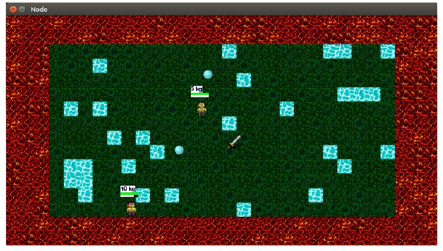
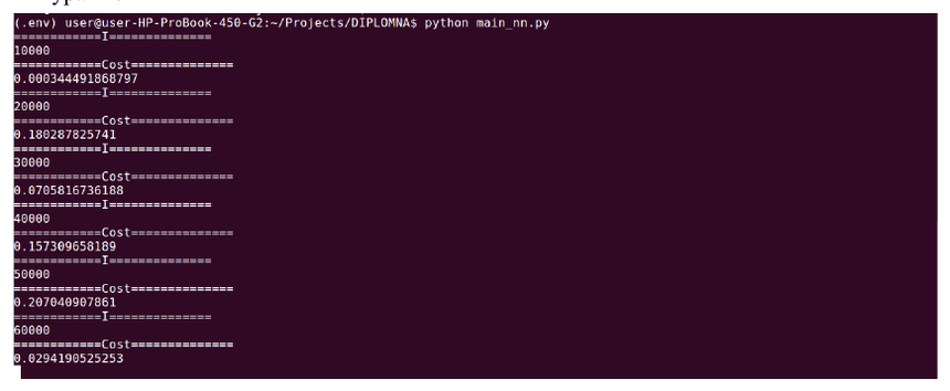
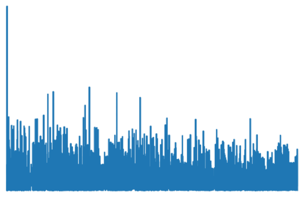
python main_nn.pyAn empty window should appear (Figure 24), and in the console, roughly every 5–10 seconds, the interim accuracy of the model is printed (Figure 25). The console text is the indicator that the algorithm is working while it learns. The window is empty because the environment's graphics are switched off during learning, which speeds it up several times over. When the learning phase ends, a graph appears showing the model's accuracy over the training time (Figure 26). At that point the graph can be analysed; when it is closed, the game starts, and the behaviour of the player controlled by the artificial intelligence, the model, can be analysed as well as its graph (Figure 27, at the top of this page).
Experimental data
Original pages 41–44
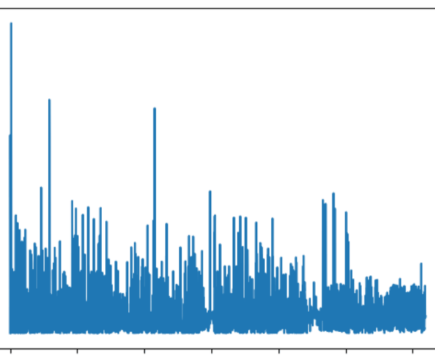
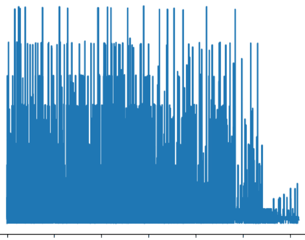
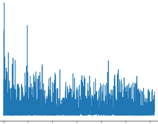
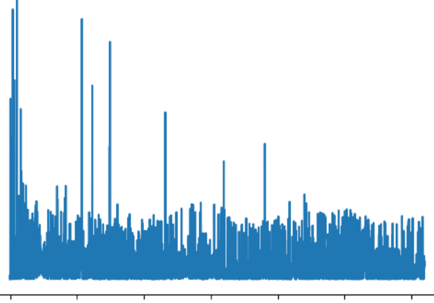
The experimental data below are shown as pairs of a table and a graph, the graph being the direct result of running the training. The horizontal axis is time, or more precisely the number of frames over which the model was trained; the vertical axis is the value of the error of the model's function. The smaller the value, the more accurate the algorithm.
| Run | Neurons per layer (1 → 5) | γ discount | lr learning rate | e greediness | train (steps) | Graph |
|---|---|---|---|---|---|---|
| Table 4 | 26 · 10 · 6 · 6 · 4 | 0.2 | 1e-4 | 0.2 | 100,000 | Figure 28 |
| Table 5 | 26 · 10 · 6 · 6 · 4 | 0.2 | 1e-2 | 0.2 | 200,000 | Figure 29 |
| Table 6 | 26 · 20 · 20 · 10 · 4 | 0.2 | 1e-4 | 0.2 | 100,000 | Figure 30 |
| Table 7 | 26 · 20 · 10 · 4 · 4 | 0.2 | 1e-5 | 0.2 | 100,000 | Figure 31 |
Conclusion
Original pages 45–46
The science of artificial intelligence occupies an ever larger part of business. The broadest interest is in the machine-learning sector: it is used widely and is an inseparable part of the algorithms for recommending goods, personalising advertising, optimising routes, computer vision, translating text and much else. The original illustrates the growth of interest in machine learning over the previous five years with a search-trends chart.
The breakthrough, however, is being made by the reinforcement-learning sector. It applies mainly to games and simulated environments, with autonomous cars as the exception. We will see the automation of ever more complex human activities, and reinforcement-learning algorithms will inevitably be used for it. They allow a model to be trained even without data and without labels, purely by specifying a reward for a given action. Two further trend charts in the original show public interest in "reinforced learning" and in "autonomous car" over five years.
Given this, we can agree that the demand for people able to build artificial intelligence that solves these problems will grow. This thesis finds its application in training those people, through the analysis of the agent's resulting behaviour in a simulated environment. Graphical representation is an indispensable tool for understanding the algorithms used in developing artificial intelligence with reinforcement learning.
Sources
Original page 47 · listed as in 2017; some links may no longer resolve
- pygame.org/wiki/about; cio.bg, "Изкуствен интелект: основни концепции и приложение в отбранителната техника"
- r/MachineLearning: Understanding Q-learning in neural networks
- CiteSeerX paper, doi 10.1.1.72.1193
- YouTube: yS5F_vm9Ahk, on sub-rewards for strategy
- YouTube: IXuHxkpO5E8, on decreasing the learning rate, a hard-coded initial estimate, and an exploration bonus
- mnemstudio.org: Path-finding Q-learning tutorial
- matplotlib.org
- Sutton & Barto, Reinforcement Learning: An Introduction, draft of June 2017
- DeepMind, Human-level control through deep reinforcement learning (Nature, 2015)
- Python docs: math
- NumPy reference
- matplotlib 2.0.2 pyplot summary
- Python docs: os
- Python docs: random
- github.com/openai/gym
- Stack Overflow: Training a neural network with reinforcement learning
- outlace.com: Reinforcement learning, part 3
- github.com/openai/gym
- Wikipedia: OpenAI
- tensorflow.org
- slant.co: TensorFlow alternatives
- virtualenv user guide
- pip user guide
Appendix
Original page 48
The source code of the application can be found at bitbucket.org/donald_ovcharov/tu.diplomna.
For a 2026 reading of that code, commit by commit, with an assessment against the DeepMind paper and a live Q-learning demo, see the companion article A Deep Q-Network from scratch.
Bachelor's thesis, Technical University of Sofia, Faculty of Computer Systems and Control, Computer and Software Engineering, defended in 2017. Supervisor M.Eng. D. Andreev.
English showcase edition prepared in 2026. Condensed where the original summarised public reference material; the author's own text, figures, tables and results are kept. Third-party figures redrawn or described.
Donald Ovcharov, founder of 402. AI research and implementation since 2017. Talk to us about AI →